Making Monte Carlo cheaper: control variates for SDE simulation

Stochastic differential equations rarely have closed-form solutions, so if you want $\mathbb{E}[g(X_T)]$ for some functional $g$ of the solution, you simulate: discretize the equation, generate many paths, average. That gives you two separate errors. Discretization contributes a bias of order $\mathcal{O}(\Delta t)$, and averaging finitely many paths contributes a statistical error of order $\mathcal{O}(N^{-1/2})$.

The second rate is the annoying one. It doesn’t care about the dimension of the problem, which is why Monte Carlo is used at all — but it is slow. Cutting the error by a factor of ten costs a hundred times more paths. Since the cost per path is fixed, buying accuracy by brute force stops being viable very quickly.

The root mean squared error of the estimator is

and $N$ sits in the denominator, but $\sigma_g$ sits in the numerator. This is the whole idea behind my seminar paper: instead of pushing $N$ up, push $\sigma_g$ down.

The setup

Take an Itô process

and approximate it with the Euler–Maruyama scheme on a uniform grid $t_n = n\,\Delta t$:

The Monte Carlo estimator $\hat{\theta}_\Delta = \frac{1}{N}\sum_i g(Y_M^{(i)})$ is unbiased for the discretized target $\mathbb{E}[g(Y_M)]$; its bias relative to the true $\mathbb{E}[g(X_T)]$ is exactly the weak error of the scheme, which for Euler–Maruyama is $\mathcal{O}(\Delta t)$. Those are two different knobs — $\Delta t$ controls the bias, and everything below is about the variance.

Control variates

The trick is to pair each simulation output $A_i$ with a second quantity $C_i$ computed on the same path, whose expectation you happen to know exactly. Then for any fixed $b$,

and averaging gives $\hat{A}(b) = \hat{A} - b(\hat{C} - \mathbb{E}[C])$. Since $\mathbb{E}[\hat{C} - \mathbb{E}[C]] = 0$, the correction term has mean zero, so the estimator stays unbiased no matter what $b$ you pick. What changes is the variance:

minimized at

Two things worth noticing. First, $b^*$ is literally the slope of a linear regression of $A$ on $C$ — the method is regressing out the part of the noise that the control can explain. Second, the payoff is entirely governed by $\rho_{CA}^2$: a control correlated at $0.5$ buys you 25% of the variance, while one correlated at $0.99$ buys you 98%. Weak controls are nearly worthless, and good ones are dramatic.

In practice $b^*$ is unknown and gets estimated from the same sample as $\hat{b} = \widehat{\text{Cov}}[C, A] / \widehat{\text{Var}}[C]$. That reintroduces a small bias of order $\mathcal{O}(1/N)$ — $\hat{b}$ and the term it multiplies are no longer independent — but it is dominated by the $\mathcal{O}(N^{-1/2})$ standard error and is normally ignored.

A small example first: estimating $\pi$

Throw points uniformly into the unit square and count how many land in the quarter disc. The scaled indicator $\psi = 4 \cdot \mathbb{1}\{x^2 + y^2 \le 1\}$ has mean $\pi$. As a control, take the average squared distance from the origin, $C = \frac{1}{m}\sum_j (x_j^2 + y_j^2)$, whose expectation is $\frac13 + \frac13 = \frac23$ — no simulation needed, just two integrals.

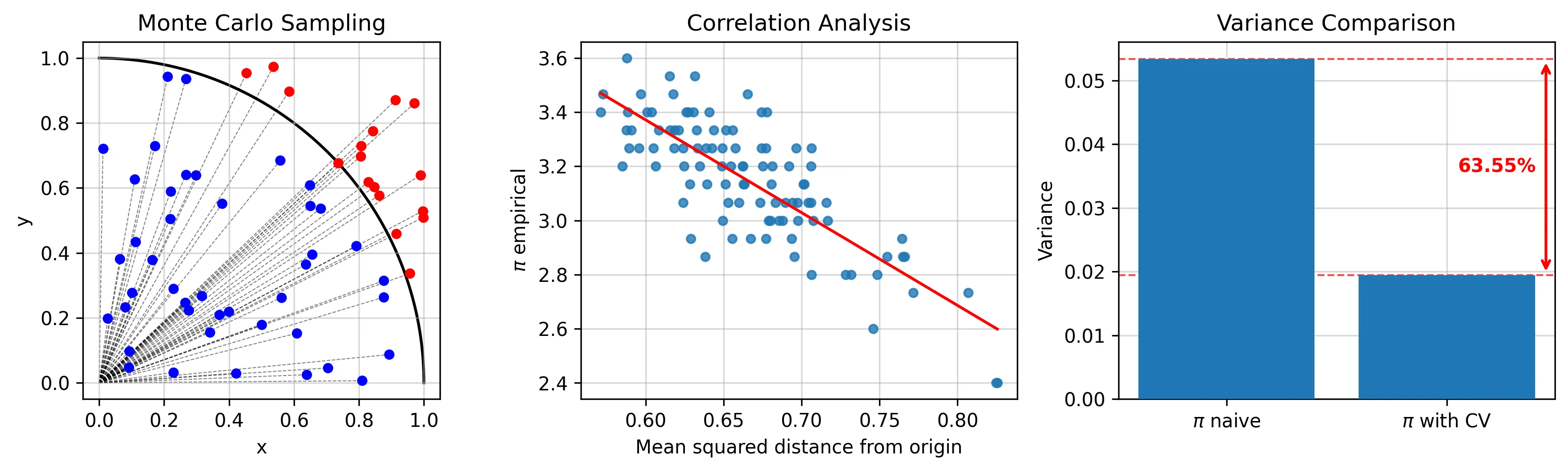
The middle panel is the point: the empirical $\pi$ and the control move together, and the fitted regression line is $\hat{b}$. Subtracting that fitted component removes about 64% of the variance with $m=100$ points per trial over $n=60$ trials — for the cost of one extra sum per point.

A martingale as the control

For SDEs there’s a natural source of controls with known expectations: martingales. A martingale satisfies $\mathbb{E}[X_t \mid \mathcal{F}_s] = X_s$, so its expectation is pinned to its starting value — the “known expectation” requirement comes for free. And if you build one from the same Brownian increments $\Delta B_n$ that drive your simulation, it picks up the same noise, which is where the correlation comes from.

The concrete case in the paper is a European call under geometric Brownian motion. The asset follows $dS_t = rS_t\,dt + \sigma S_t\,dB_t$, and the target is the discounted payoff $A = e^{-rT}\max(S_T - K, 0)$. (There is a closed-form answer here, of course; the point is to pretend there isn’t and check the method against something verifiable.)

Consider the discounted price $Z_t = e^{-rt}S_t$ and apply Itô’s formula. Since $h(t,x) = e^{-rt}x$ is linear in $x$, the second-order term vanishes:

The drift cancels exactly. What’s left is a pure Itô integral, which is a martingale, so $\mathbb{E}[Z_T] = Z_0 = S_0$.

There is one detail that matters in practice. The simulation doesn’t produce $S_T$, it produces the Euler–Maruyama approximation $Y_M$, so the control that actually gets used is $C_\Delta = e^{-rT}Y_M$ — and its expectation is not $S_0$. Taking expectations through the scheme with $\mathbb{E}[\Delta B_n] = 0$ gives

which is again known exactly, in closed form. Using the discrete expectation rather than the continuous one is what keeps the corrected estimator unbiased with respect to the discretized target instead of picking up a fresh $\mathcal{O}(\Delta t)$ bias through the back door.

What it does, and where it stops working

Simulating $N = 10{,}000$ paths with $M = 100$ steps, $S_0 = 50$, $r = 0.05$, $T = 0.25$, $\sigma = 0.3$, and sweeping the strike:

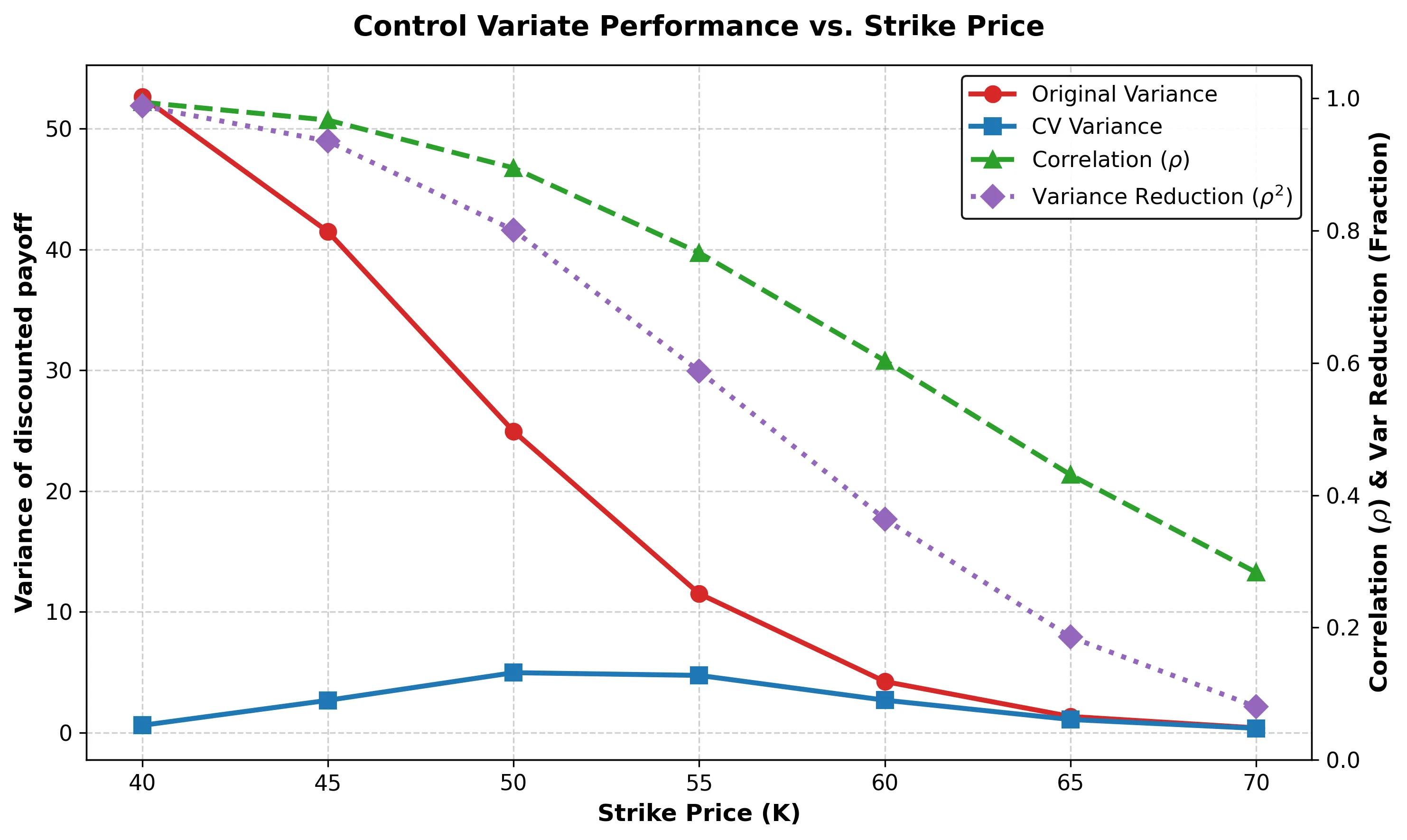
Deep in the money, the control removes 99% of the variance — the same accuracy for roughly 1% of the paths. That is a much better deal than anything you get by increasing $N$.

But the effect decays fast, and the reason is structural rather than numerical. When $K$ is well below $S_0$, the option almost always pays out, the payoff is essentially $e^{-rT}S_T$ minus a constant, and the discounted price tracks it almost perfectly. As $K$ rises, the $\max(\cdot, 0)$ starts clipping more and more paths to zero. The payoff stops being a linear function of the terminal price, the correlation collapses, and with it — quadratically — the benefit. By $K = 70$ the control is doing almost nothing.

That failure mode is what makes the last observation interesting. The optimal coefficient is a regression slope, and the method is a linear projection onto a single hand-picked control. Nothing forces it to stay linear or hand-picked: for payoffs too awkward to handle analytically, you could train a model to produce a control that is highly correlated with the payoff and whose expectation is still known. That’s the direction I’d like to take this next.

Full write-up, with the definitions, proofs and references: Monte Carlo Simulation of SDEs and Variance Reduction via Control Variates (PDF).